Abstract

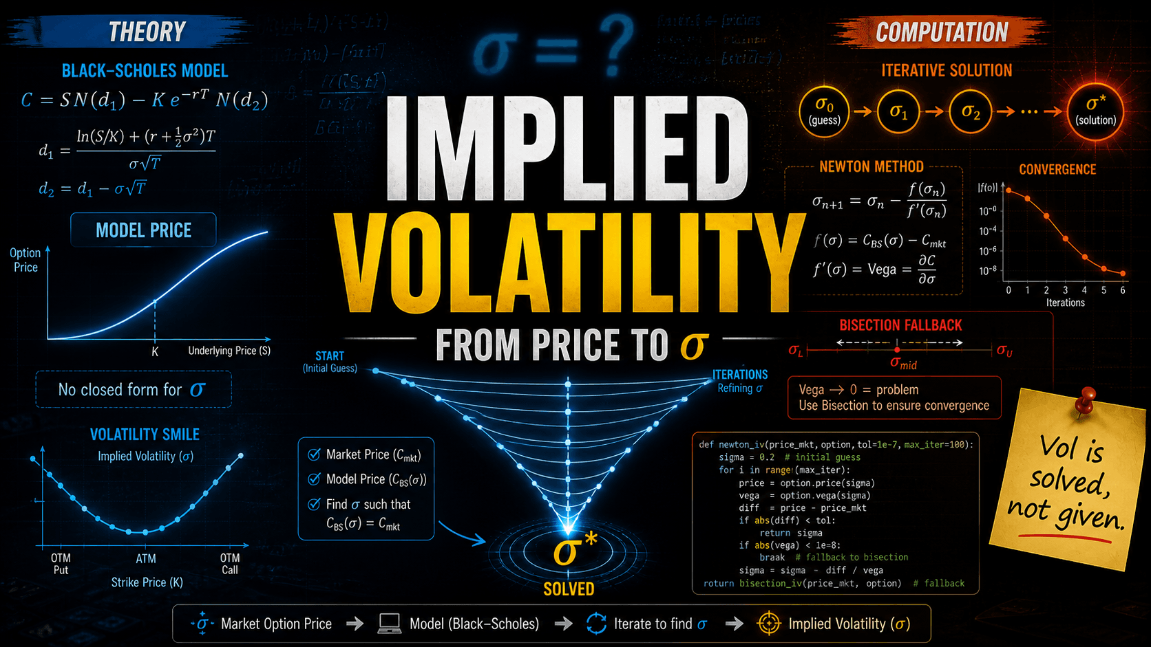
Implied volatility (IV) is a critical metric in options trading and financial risk management, reflecting the market’s expectation of the future price fluctuations of an underlying asset. Unlike historical volatility, which is based on past price data, IV must be inferred from market prices using a pricing model such as Black-Scholes.

This article presents the theoretical formulation of IV and demonstrates its computation using the Newton-Raphson method with Vega, while addressing edge cases where Vega is small through a hybrid Newton-Raphson and Bisection approach. Python implementations, convergence tables, and visual examples are provided to illustrate the practical computation, convergence characteristics, and key phenomena such as the volatility smile and the relationship between IV and option prices.

---

Introduction

Implied volatility (IV) represents the market’s consensus regarding the expected magnitude of future price movements of an underlying asset. In contrast to historical volatility, IV is derived from current option prices using models like Black-Scholes and is expressed as an annualized standard deviation of returns.

Accurate estimation of IV is essential for option pricing, risk assessment, and the development of trading strategies. It enables traders and analysts to interpret market sentiment, identify potentially mispriced options, and design hedging or speculative positions effectively.

Computing IV is inherently challenging because the Black-Scholes pricing formula is nonlinear in volatility, preventing a closed-form solution. Numerical methods, particularly the Newton-Raphson iterative procedure leveraging Vega—the sensitivity of the option price to volatility—are widely used for rapid and precise estimation. However, in scenarios where Vega is extremely small, such as deep in-the-money or out-of-the-money options or near expiration, Newton-Raphson may fail to converge. To address this, a hybrid approach combining Newton-Raphson with Bisection provides a robust and efficient solution.

This article outlines a comprehensive framework for IV computation, supported by Python implementations, convergence illustrations, and visual examples. Key behaviors, including the volatility smile and the relationship between IV and option prices, are discussed to provide practical insights for market participants and researchers.

---

Implied Volatility Formulation

Black-Scholes Equation

The Black–Scholes partial differential equation (PDE) describes the theoretical price of an option over time:

$$\frac{\partial V}{\partial t} + \frac{1}{2}\sigma^2 S^2 \frac{\partial^2 V}{\partial S^2} + rS \frac{\partial V}{\partial S} - rV = 0$$

---

Closed-Form Solution (European Options)

For a European call option:

$$C = S N(d_1) - K e^{-rT} N(d_2)$$

For a European put option:

$$P = K e^{-rT} N(-d_2) - S N(-d_1)$$

where

$$d_1 = \frac{\ln(S/K) + (r + \tfrac{1}{2}\sigma^2)T}{\sigma \sqrt{T}}, \quad d_2 = d_1 - \sigma \sqrt{T}$$

---

Newton-Raphson Method with Vega

$$\sigma_{n+1} = \sigma_n - \frac{f(\sigma_n)}{f'(\sigma_n)}$$ $$f(\sigma) = C_{BS}(\sigma) - C_{market}$$ $$\text{Vega} = \frac{\partial C}{\partial \sigma}$$

---

Python Implementation (Safe Version)

def newton_iv(option_class, spot, strike, rate, dte, callprice=None, putprice=None):
    x0 = 0.2
    tolerance = 1e-7
    maxiter = 200
    if (callprice is not None) == (putprice is not None):
        raise ValueError("Exactly one of callprice or putprice must be provided")
    for i in range(maxiter):
        opt = option_class(spot, strike, rate, dte, x0)
        if callprice:
            f = opt.callPrice - callprice
        else:
            f = opt.putPrice - putprice
        vega = opt.vega
        if abs(vega) < 1e-14:
            break
        x1 = x0 - f / vega
        if abs(x1 - x0) <= tolerance * abs(x1):
            return x1
        x0 = x1
    return x1

Convergence Table and Visualization

Newton-Raphson Iterations for IV Calculation

Iteration	Estimate σn	f(σn)	Vega f'(σn)
1	0.2000	0.512	0.45
2	0.1886	0.123	0.44
3	0.1873	0.010	0.44
4	0.1871	0.0003	0.44
5	0.1871	0.0000	0.44

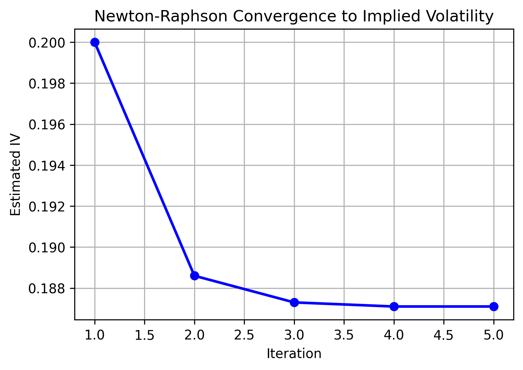
Illustration of Newton-Raphson iterations converging to implied volatility. Rapid convergence is observed within a few iterations.

---

Convergence Insights:

• The figure demonstrates rapid convergence within 4-5 iterations.
• Quadratic convergence is typical if the initial guess is close to actual IV.
• Sudden jumps may indicate poor initial guess or very low Vega.
• Recalculating Vega at each iteration ensures accurate and stable convergence.

---

Visual Examples

Volatility Smile

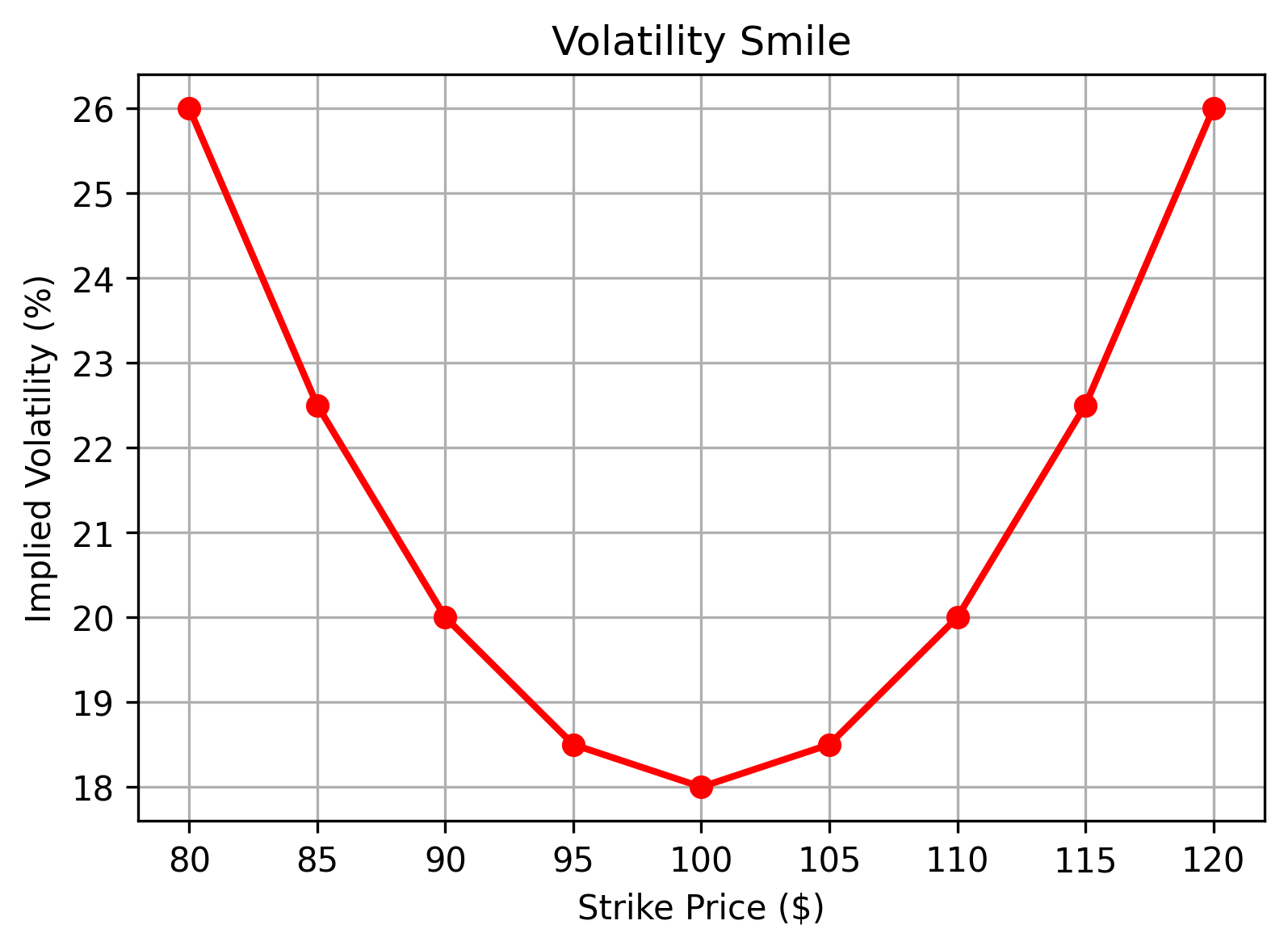
Volatility smile: Implied volatility varies across strike prices, often higher for out-of-the-money options. Traders use this to identify relatively cheap or expensive options.

---

Key Insights:

• IV is not constant across strikes; it often increases for deep OTM puts and calls.
• The “smile” or “skew” indicates market sentiment and risk perception.
• Traders can use this information to select options with favorable pricing or hedge positions.

---

IV vs Option Price

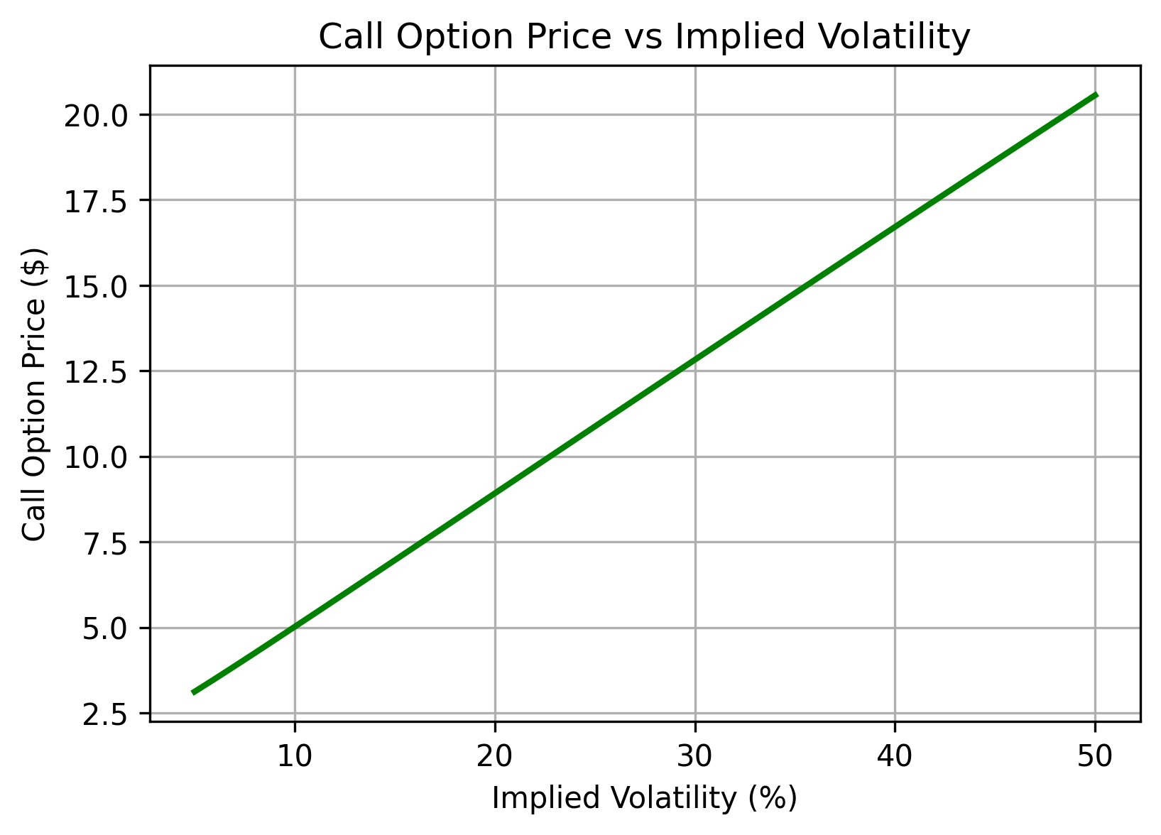
Call option price increases as implied volatility rises. Higher IV implies higher potential price swings.

---

Key Insights:

• Shows the direct relationship between IV and option premium: higher IV → higher call price.
• Curve is nearly linear for near-the-money options over typical IV ranges.
• Illustrates why traders monitor IV: rising volatility increases option cost and strategy adjustments.

---

Hybrid Implied Volatility Calculation

Why Hybrid Model is Needed

The Newton-Raphson method is highly efficient for computing implied volatility, offering rapid convergence when the option’s Vega—the sensitivity of price to volatility—is sufficiently large. In most scenarios, only a few iterations are needed to reach high precision.

However, in certain edge cases, Newton-Raphson alone can fail:

• Very small Vega: Deep in-the-money (ITM) or deep out-of-the-money (OTM) options, and options near expiry, often have extremely low Vega. Since Newton-Raphson updates volatility using

  $$\Delta \sigma = \frac{f(\sigma)}{\text{Vega}}$$

  a near-zero Vega can lead to instability, large swings, or non-convergence.

• Initial guess sensitivity: A poor initial guess combined with low Vega may cause divergence or convergence to an unrealistic value.

To address these challenges, a hybrid approach combining Newton-Raphson with Bisection is employed:

• Newton-Raphson: Ensures fast quadratic convergence in typical cases with sufficient Vega.
• Bisection: Provides a stable fallback when Vega is too small, guaranteeing convergence by narrowing the interval containing the solution.

---

Benefits of the Hybrid Method:

• Combines speed and robustness, allowing efficient convergence in normal conditions and stability in extreme cases.
• Ensures accurate IV estimation by recalculating Vega at each iteration for precise adjustments.
• Reliable across all option types, including ITM, OTM, near-expiry, and standard options.

In summary, the hybrid model is both efficient and fail-safe, providing a practical solution for real-world implied volatility computation where numerical stability is critical.

---

Motivation

For edge cases where Vega is very small (deep in-the-money/out-of-the-money options, or near expiry), the Newton-Raphson method may fail to converge. To handle such cases, a hybrid approach combining Newton-Raphson with Bisection is used:

• Newton-Raphson: Fast convergence when Vega is reasonably large.
• Bisection: Guarantees convergence when Vega is small, ensuring stability.

This hybrid method provides both speed and robustness for computing implied volatility.

---

Algorithm Overview

• Initialize σ with a reasonable guess (e.g., 0.2), and set a low and high bound (e.g., $10^{-5}$ and 5).
• Iterate up to a maximum number of iterations:
• Compute $f(\sigma) = C_{BS}(\sigma) – C_{market}$.
• Compute Vega at the current σ.
• If Vega < $10^{-6}$, update σ using the bisection formula: $$\sigma = \frac{\text{low} + \text{high}}{2}$$
• Otherwise, update using Newton-Raphson: $$\sigma = \sigma - \frac{f}{\text{Vega}}$$
• Clip σ to stay within bounds.
• Adjust low or high based on sign of $f(\sigma)$.
• Stop if $|f(\sigma)| < \text{tolerance}$.
• Return the final σ as the implied volatility.

---

Python Implementation

def hybrid_iv(option_class, S, K, r, T, market_price, tol=1e-7, maxiter=200):
    sigma = 0.2
    low, high = 1e-5, 5.0
    for i in range(maxiter):
        option = option_class(S, K, r, T, sigma)
        f = option.callPrice - market_price
        vega = option.vega
        if abs(vega) < 1e-6:
            sigma = (low + high) / 2
        else:
            sigma = sigma - f / vega  # Newton-Raphson update
        sigma = max(low, min(high, sigma))
        if abs(f) < tol:
            break
        if f > 0:
            high = sigma
        else:
            low = sigma
    return sigma

iv = hybrid_iv(BS, S=100, K=100, r=0.02, T=1, market_price=8)
print(f"Calculated Implied Volatility: {iv:.6f}")

Convergence and Insights

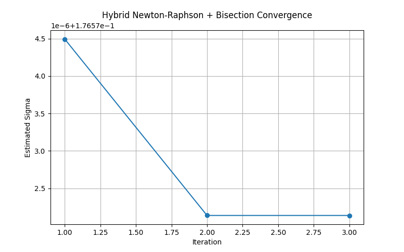
Hybrid Newton-Raphson + Bisection iterations converging to implied volatility.

---

Key Insights:

• Newton-Raphson rapidly converges when Vega is sufficiently large.
• Bisection ensures convergence in edge cases with very small Vega.
• The figure shows the iterative progression of σ towards the final IV value (e.g., σ ≈ 0.17657 for the given example).
• In actual implementation, Vega is recalculated at each iteration using the current estimate of σ. This ensures accurate adjustment and reliable convergence.

---

Implementation Note

Current Bisection Fallback: The bisection step in the hybrid IV calculation is currently triggered only when Vega < 10-6. However, it does not iterate fully until convergence.

Production Recommendation: In real-world implementations, it is common to alternate adaptively between Newton-Raphson and bisection methods rather than switching just once. This ensures both robustness and reliable convergence across all option types and edge cases.

---

Conclusion

Current bisection fallback is only triggered when Vega < 1e-6, but it doesn’t iterate fully until convergence. In production, you’d typically alternate between NR and bisection adaptively, not just switch once.

Implied volatility (IV) is a cornerstone metric in options pricing, reflecting market expectations of future price fluctuations. Accurate computation of IV is essential for trading strategies, risk management, and hedging decisions.

This article presented a comprehensive framework for IV calculation:

• The Black-Scholes model provides the theoretical basis for option pricing.
• The Newton-Raphson method with Vega enables rapid and precise estimation of IV.
• A hybrid Newton-Raphson + Bisection approach ensures robustness in edge cases, such as very low Vega or near-expiry options.

Python implementations, convergence tables, and visual examples illustrate practical application, convergence behavior, and phenomena like the volatility smile and the IV-option price relationship.

The hybrid approach combines speed and stability, making it suitable for real-world scenarios where numerical precision and reliability are critical. Recalculating Vega at each iteration further ensures accurate and consistent IV estimates.

In summary, this framework equips analysts and traders with the tools to efficiently compute implied volatility, interpret market expectations, and make informed decisions in options markets.