Nonlinear Signal Transforms and the Skewness Trade-off
May 02, 2026 - Tribhuven Bisen
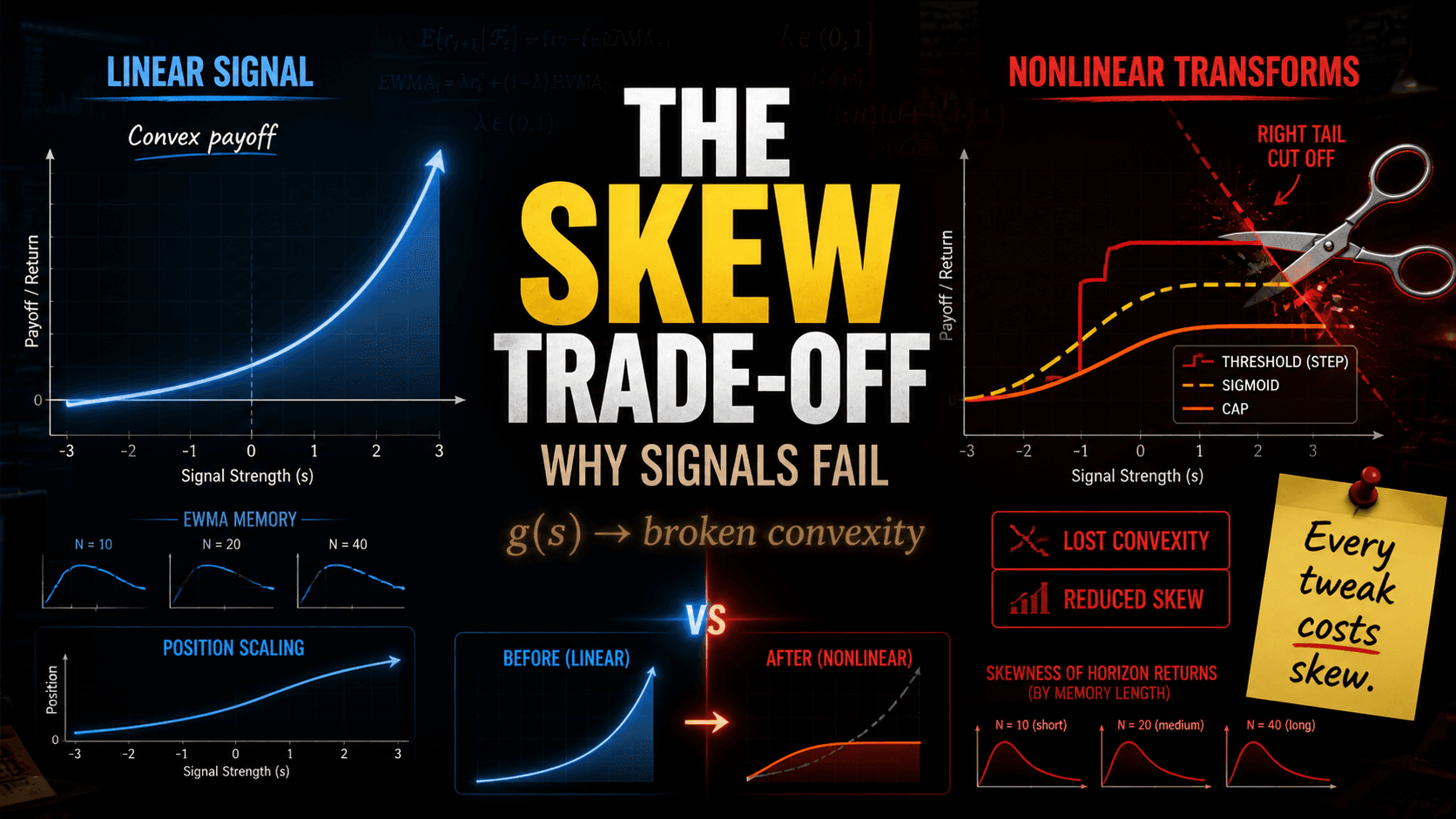
A practical accounting of what we give up when we cap, threshold, or smooth momentum signals: skewness is the tax we pay for trend insurance.
Every practitioner who has shipped a trend-following strategy has, at some point, looked at the raw signal and decided it needed help. The signal is too jumpy, so we smooth it. It produces small positions on noise, so we threshold it. It blows up in fat-tailed regimes, so we cap it. Each decision feels like a refinement, and each one quietly removes a slice of the property that made trend-following worth running in the first place.
That property is positive skew. Trend strategies often lose small and frequently, then win large and rarely. Investors do not pay for the Sharpe ratio alone; they pay for convexity. The straddle-like payoff profile historically associated with long-horizon trend programs is the economic case for the style.
This note walks through three common nonlinear transforms applied to a momentum signal, then measures how each one degrades skewness across horizons:
- Step function with threshold
- Sigmoid (smooth saturation)
- Reverse sigmoid (bell-shaped exposure)
The conclusion is uncomfortable but practical: almost any deviation from a linear signal lowers skew, and the more "intuitive" the modification, the more aggressively it can do so.
1) The skew you did not expect
Start with IID standard normal returns:
Build an exponentially weighted signal and trade it:
Define horizon return:
Even with symmetric input returns, the strategy can generate positive skew through interaction terms in the signal recursion. In simulation, skewness rises with horizon, peaks, and then decays; the peak location and amplitude depend on EWMA memory length.
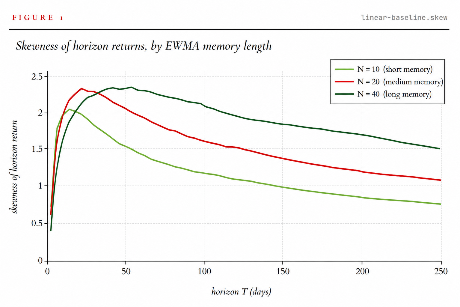
Figure 1: Longer memory shifts the skew peak to later horizons and can increase peak skew before eventual decay.
Two practical implications:
- Measurement horizon matters. The same strategy can look far more skewed on quarterly returns than on daily returns.
- Linear EWMA is the skew-preserving baseline. Most post-processing transforms move away from this baseline by reducing convexity.
The linear signal is the ceiling. Every transform we add is paid in skew.
2) Three things we do to signals
2.1 Step transform (thresholding)
Ignore weak signals and trade only when conviction crosses a threshold:
This controls churn around zero and simplifies execution, but it also removes size scaling in strong trends.
2.2 Sigmoid transform (smooth cap)
Allow all signals but saturate large exposures:
This is common in modern systematic pipelines and ML-style position layers.
2.3 Reverse sigmoid (mid-strength preference)
Emphasize moderate signals and de-emphasize extremes:
The intuition is "extremes may be noisy," but this can be costly for convexity.
3) Measuring the skew tax
Hold the base signal fixed (EWMA, ), apply each transform, and recompute skewness by horizon.
Step transform impact
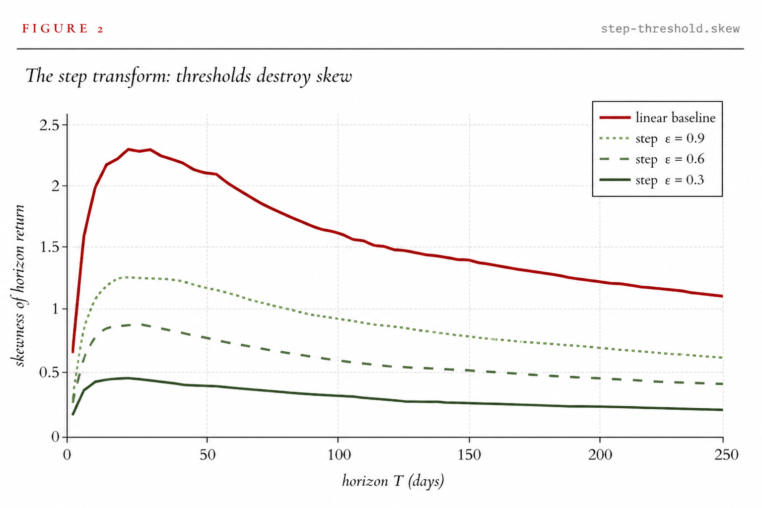
Figure 2: Tight thresholds compress right-tail outcomes sharply. Lower turnover can come at a large convexity cost.
The step transform is especially punitive because it kills the strategy's ability to scale position with trend strength. A mild trend and a roaring trend can receive similar position size once thresholding is imposed.
Sigmoid vs reverse sigmoid
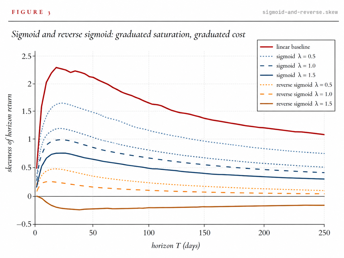
Figure 3: Sigmoid reduces skew gradually as saturation tightens; reverse sigmoid can become deeply destructive and even push skew negative at stronger settings.
Observed ranking in convexity retention (best to worst):
- Linear baseline
- Sigmoid (gentle settings)
- Step transform
- Reverse sigmoid (strong settings can invert skew sign)
4) Why this happens
In one line: trend skew is the covariance between position size and trend strength.
Any transform that weakens the mapping from signal magnitude to position magnitude weakens that covariance:
- Step transform: removes scaling abruptly
- Sigmoid: attenuates scaling monotonically
- Reverse sigmoid: can reverse scaling in tails
So there is no non-trivial cap/threshold transform that keeps skew fully intact.
Cap position responsiveness, and you cap convexity.
5) Design implications for live systems
If you must cap
Prefer a sigmoid. Its knob is interpretable and gives a smoother risk-convexity trade-off.
If you must threshold
Threshold signal changes (rebalance trigger) rather than absolute signal levels. This controls turnover more directly while preserving more tail behavior.
Avoid reverse sigmoid sizing in production trend books
If extreme signals seem unreliable, fix the estimation upstream (robust features, regime handling, data quality), not through a tail-punishing position map.
Audit skew at investor horizon
Daily diagnostics are not enough. Measure skew where your investors experience returns (monthly/quarterly windows).
6) The deeper point
Complex architectures often stack multiple nonlinear layers over an essentially linear trend engine. Each layer may be defensible in isolation, but each can also tax convexity. If reported Sharpe improves mostly through variance suppression, you may be financing that improvement by selling the right tail your mandate was meant to deliver.
The right decision is not "never transform." It is to treat skew as a budgeted resource and spend it only when the operational benefit is explicit, measured, and agreed.
Methods
- Monte Carlo simulation on horizon grid
- EWMA recursion:
- Burn-in applied before measurement windows
- Skewness estimated per horizon and compared across transforms
References
- Bouchaud, J.-P. & Potters, M. — trend-following and skewness mechanics
- Lempérière, Deremble, Seager, Potters, Bouchaud (2014) — two centuries of trend following
- Fung, W. & Hsieh, D. (2001) — trend follower risk structure
- Bruder, B. & Gaussel, N. — dynamic strategy risk-return analysis
- Martin, R. & Zou, H. — momentum and convexity decomposition (as discussed in practitioner literature)