1 What is PnL Attribution?

PnL attribution is used to answer:

• What drove today’s PnL? (market factors vs time vs model effects)
• How good were my hedges? (did sensitivities behave as expected?)

It decomposes portfolio PnL into components such as theta (time decay), delta (underlying move), gamma (convexity), and vega (volatility move). Beyond desk-level risk management, attribution is also used as a diagnostic for model quality: do the sensitivities explain realized PnL?

---

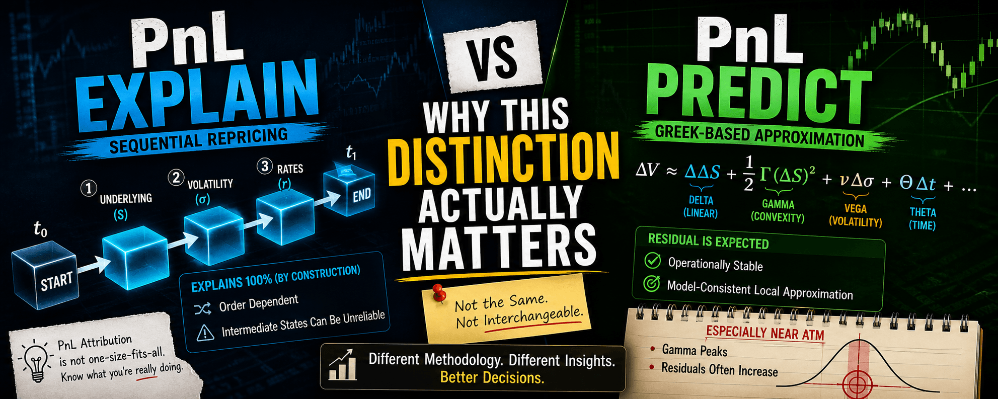
2 Explained vs Predict

2.1 PnL Explain (Sequential / Path-Based)

Idea: Move market variables one-by-one and reprice after each move. A typical sequence:

$$(t) \rightarrow (S) \rightarrow (\sigma) \rightarrow (r) \rightarrow \cdots$$

The incremental price change after each move is attributed to the variable moved at that step.

Key properties

• Fully attributes PnL by construction (sum of steps equals total repricing PnL).
• Order-dependent: different sequences can produce different decompositions.
• Intermediate states can be unrealistic: mixing “yesterday” and “today” inputs can create inconsistent states.
• Theta is special: whether time is moved first or last is often the biggest methodological decision.

---

2.2 PnL Predict (Greek / Sensitivity-Based)

Idea: Use start-of-day (or previous close) sensitivities and multiply by observed market moves:

$$\Delta V \approx \Delta \Delta S + \tfrac{1}{2} \Gamma (\Delta S)^2 + \nu \Delta \sigma + \Theta \Delta t + \cdots$$

where Δ is delta, Γ gamma, ν vega, and Θ theta.

Key properties

• Operationally stable and easy to implement.
• Model-consistent: a local Taylor approximation around a reference state.
• Residual is expected: not all PnL is explained due to nonlinearity and missing higher-order terms.

---

3 The Role of Theta

Theta is not a market quote; it is the effect of time passing. In PnL Explain, the question “move time first or last?” matters because it changes the repricing state used for subsequent moves. In practice, firms adopt and enforce a convention to avoid inconsistent “mix-and-match” states that can destabilize repricing.

---

4 Explain vs Predict: Summary Comparison

Aspect	PnL Explain	PnL Predict
Method	Sequential repricing after moving variables one-by-one	Greeks × observed moves (local Taylor approximation)
Explains 100%?	Yes (by construction)	No (residual is expected)
Order sensitivity	Yes (depends on attribution path)	No (single expansion around a reference state)
Operational stability	Can be fragile if intermediate states are inconsistent	Stable; always produces a number
Typical use	Desk reporting, forensic analysis	Daily monitoring, hedge/model diagnostics

Table 1: Conceptual comparison of PnL Explain and PnL Predict.

---

5 Why Residual Often Peaks Near ATM (Gamma Effect)

A common observation is that discrepancies between predicted and realized PnL often concentrate near-the-money (ATM), where options typically have the highest gamma. Gamma contributes a nonlinear term:

$$\text{Gamma PnL} \approx \tfrac{1}{2} \Gamma (\Delta S)^2$$

If gamma is stale, mis-estimated, or higher-order effects matter, residuals often increase where convexity is largest.

---

6 Minimal Worked Template (Plug-in Numbers)

Let $V_{t-1}$ be the reference price and $V_t$ the price after the market move:

$$\text{Realized PnL} = V_t - V_{t-1}$$

A second-order PnL Predict approximation:

$$\text{Predicted PnL} = \Delta \Delta S + \tfrac{1}{2} \Gamma (\Delta S)^2 + \nu \Delta \sigma + \Theta \Delta t$$

Residual definitions:

$$\text{Residual} = \text{Realized PnL} - \text{Predicted PnL}$$ $$\text{Residual \%} = \left(\frac{\text{Residual}}{\text{Realized PnL}}\right) \times 100$$

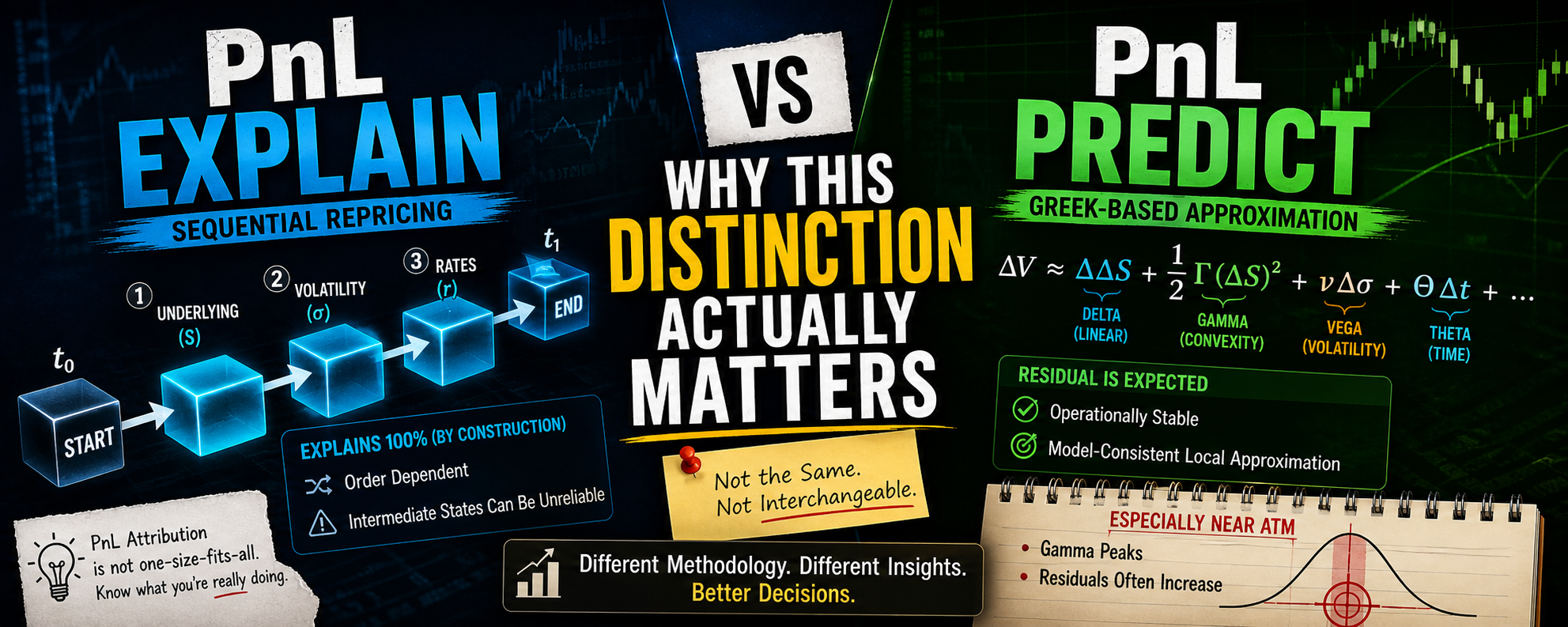
Figure 1: Stylized intuition: gamma peaks near ATM, and residuals often increase where convexity dominates.

---

7 PnL Explained vs PnL Predicted: Side-by-Side

The two methodologies often produce similar totals, but the internal decomposition can differ materially, especially in how convexity (gamma) and volatility (vega) effects appear.

Component	ATM	OTM	ITM	Fly
PnL Explain (Sequential Repricing)
Underlying (Delta)	0.72	0.31	0.88	–
Theta	-0.03	-0.02	-0.02	–
Vega	-0.41	-0.27	-0.32	–
Total Explained	0.28	0.02	0.54	–
Unexplained	0.00	0.00	0.00	–
PnL Predict (Greek-Based)
Delta + Gamma	0.71	0.32	0.87	–
Theta	-0.03	-0.02	-0.02	–
Vega	-0.39	-0.28	-0.31	–
Total Predicted	0.29	0.02	0.54	–
Unexplained (Abs)	-0.01	0.002	0.004	–
Unexplained (%)	-3.6%	10.0%	0.7%	–

Table 2: PnL Explain vs PnL Predict: totals remain close, but component-level differences especially Gamma and Vega generate residuals.

---

Interpretation. PnL Explain reproduces the realized PnL exactly because it is constructed by sequentially repricing the portfolio through the chosen path of market moves. By design, all effects are fully allocated and no residual remains.

PnL Predict, in contrast, uses a local sensitivity (Greek-based) approximation around the initial state. It therefore captures the first-order and selected second-order effects of market moves, but cannot perfectly reproduce nonlinear or path-dependent behavior. As a result, small residuals are natural and informative rather than problematic.

In the table, the largest mismatch appears around ATM, where gamma is highest and convexity effects dominate. OTM and ITM options, with lower gamma, show much smaller discrepancies. Differences in Vega attribution also contribute, since volatility sensitivity itself changes as the underlying and time move.

Hence, the gap between explained and predicted PnL should be read as a diagnostic: small, stable residuals indicate a well-specified model and effective hedging, while growing or unstable residuals signal increasing nonlinearity, missing higher-order effects, or model–market inconsistency.

---

8 Key Takeaways

• PnL Explain is a sequential repricing story: it can fully attribute PnL, but the decomposition depends on the chosen path.
• PnL Predict is a sensitivity story: it is operationally robust, but typically leaves a residual due to nonlinearity and missing terms.
• Theta governance (time first vs last) is one of the most consequential choices in sequential explain frameworks.
• Gamma drives nonlinear PnL: discrepancies often concentrate near ATM where convexity is highest.