Statistical Tests for Mean Reversion (Stationarity)
Apr 20, 2026 - Tribhuven Bisen
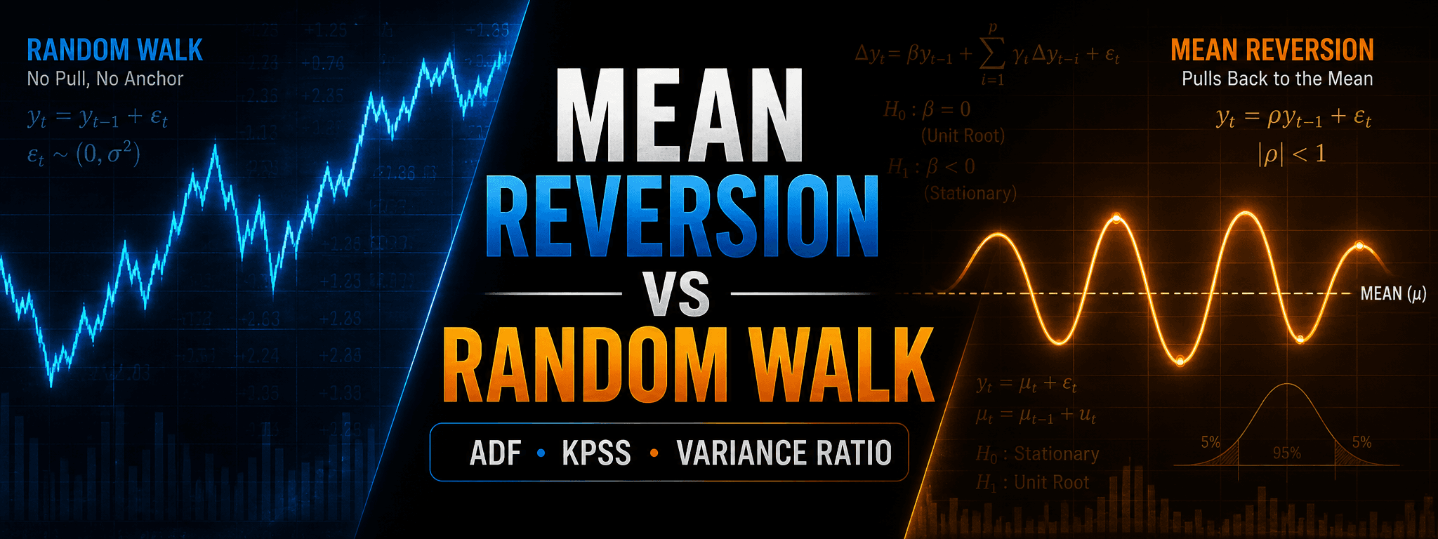
A random walk drifts without a restoring force, while a mean-reverting process pulls back toward a central level, making stationarity crucial for applying standard statistical models.
ADF, KPSS, Variance Ratio, and the Practical Issues You Actually Run Into
1. Context and the Basic Distinction
Let me start with the obvious thing that people think they understand until they actually try to trade it: a random walk is very different from something that is mean reverting.
A random walk wanders. If it goes up for a while, it can stay up for a long time. If it crosses the mean again, that can just be chance. Importantly, being far from the mean does not create a stronger pull back.
A mean reverting process is centered around some level, and the further away it gets, the stronger the expected pull back. This is the difference between something that crosses the mean rarely and something that crosses it many times.
The classic econometric framing is: many of the statistics you want to use require stationarity. If something is a random walk, you typically difference it first. If it is already stationary, you can regress it, fit AR models, and so on, without everything falling apart.
Two canonical toy models:
Random walk (unit root).
Mean reversion (AR(1), |ρ| < 1)
The whole point of the tests below is to distinguish “ρ = 1” from “ρ < 1” in a statistically disciplined way.
2. Augmented Dickey–Fuller (ADF) Test
The ADF test is the standard workhorse. Conceptually it is very simple: we regress changes on lagged levels and ask whether the level term has a negative coefficient.
Start from an AR(1):
Subtract :
Define , so
If then , and you have:
which is exactly the “increments are white noise” property of a random walk.
The augmented form adds lagged differences to mop up autocorrelation in the residuals:
2.1. Hypotheses
ADF is usually written as:
2.2. The part people get wrong: it is not a Student-t test
Even though the regression looks like a normal regression, the test statistic under H0 does not follow a Student t distribution. It follows a Dickey–Fuller type distribution. That is why ADF uses special critical values.
If you treat it like a standard t-test, you are going to fool yourself.
2.3. Choosing the lag length p
You have to choose p. Different p gives you a different test. The standard practice is to pick p by minimizing an information criterion such as AIC or BIC.
AIC.
BIC.
Here L is the likelihood, k is the number of estimated parameters, and T is sample size. AIC and BIC are both “goodness of fit minus a penalty.” They are conceptually similar to how people think about cross-validation: you do not just maximize fit, you penalize complexity.
You can pick lags visually using ACF/PACF rules of thumb. People do that. But if you’re running systematic tests, letting the routine pick p by AIC/BIC is a perfectly reasonable default.
2.4. Python example (ADF with autolag AIC)
import numpy as np
from statsmodels.tsa.stattools import adfuller

np.random.seed(0)

# Example 1: random walk
y_rw = np.cumsum(np.random.randn(2000))

# Example 2: AR(1) mean reverting
eps = np.random.randn(2000)
rho = 0.95
y_ar = np.zeros_like(eps)
for t in range(1, len(eps)):
    y_ar[t] = rho * y_ar[t-1] + eps[t]

for name, y in [("Random Walk", y_rw), ("AR(1) Mean Reverting", y_ar)]:
    stat, pval, used_lag, nobs, crit, icbest = adfuller(y, autolag="AIC")
    print("\n---", name, "---")
    print("ADF stat:", stat)
    print("p-value:", pval)
    print("lags used:", used_lag)
    print("nobs:", nobs)
    print("crit:", crit)
In trading I am not religious about the 5% line. I care whether the series is clearly mean reverting or it is basically a random walk. A p-value that barely tips under a threshold is not the same thing as a statistic that is strongly on one side.
3. Why the t-statistic fails in time series unit-root regressions
In a textbook regression, you write:
and you compare to a Student-t distribution.
In unit root settings, the asymptotics are different. Under the unit root null, the process behaves like Brownian motion in the limit. The distribution of the statistic depends on functionals of Brownian motion, not a Student-t.
One way to write the limiting idea (schematically) is that you get ratios of integrals involving Brownian motion :
which is not the same object as the usual regression t-statistic limit.
So: use the Dickey–Fuller critical values. That is the point of the test.
4. KPSS: Reversing the Null Hypothesis
KPSS is useful because it flips the null and the alternative compared to ADF.
ADF says: assume unit root, try to reject it. KPSS says: assume stationarity, try to reject it.
The model can be written as:
If , then is constant and is stationary around a mean. If , then wanders and you have a unit root type behavior.
Operationally, KPSS is built from residual partial sums. Regress on a constant (or constant+trend), take residuals , define partial sums:
Then the statistic is:
where is an estimate of the long-run variance.
4.1. Hypotheses
4.2. Python example (KPSS)
from statsmodels.tsa.stattools import kpss

# Using the same y_rw and y_ar from earlier
for name, y in [("Random Walk", y_rw), ("AR(1) Mean Reverting", y_ar)]:
    stat, pval, lags, crit = kpss(y, regression="c", nlags="auto")
    print("\n---", name, "---")
    print("KPSS stat:", stat)
    print("p-value:", pval)
    print("lags used:", lags)
    print("crit:", crit)
How I actually use it.
I like ADF and KPSS together because they are complementary. If ADF fails to reject a unit root and KPSS rejects stationarity, you are not looking at mean reversion. If both are ambiguous, you are probably in the grey zone, and you should stop pretending a binary label is going to save you.
5. Variance Ratio Test (Lo–MacKinlay)
Variance ratio is more intuitive than people give it credit for. It is based on scaling properties of a random walk:
If is a random walk, then:
Define:
Interpretation:
The reason I like this test is that you can compute it across multiple horizons k and see the structure. It is a very visual diagnostic.
5.1. Python example (simple variance ratio across horizons)
import numpy as np

def variance_ratio(y, k):
    y = np.asarray(y)
    dy1 = np.diff(y)
    dyk = y[k:] - y[:-k]
    return np.var(dyk, ddof=1) / (k * np.var(dy1, ddof=1))

ks = [2, 5, 10, 20, 50]

for name, y in [("Random Walk", y_rw), ("AR(1) Mean Reverting", y_ar)]:
    print("\n---", name, "---")
    for k in ks:
        print(f"k={k:>3d}  VR={variance_ratio(y, k):.4f}")
In practice, I care less about whether VR(k) is “statistically significant” at 5% and more about how far it is from one. If it is barely below one, it is usually not worth trading. If it is meaningfully below one, you often see better risk-adjusted behavior. This is not magic: stronger negative autocorrelation is a stronger economic effect.
6. Lag Length Choice: AIC, BIC, PACF (and why it matters)
In ADF, the whole “augmented” part is the lagged differences:
If you use too few lags, you leave autocorrelation in residuals and contaminate the test. If you use too many, you eat degrees of freedom and lose power.
There are multiple ways to pick p:
- AIC/BIC: automated, objective-ish, and widely used in practice.
- PACF: common visual heuristic for AR order selection; people do this.
I would not pretend there is a universal “correct” p. If your series is high frequency, your effective dynamics are different from daily. Use AIC/BIC as a default, and if you are building a strategy, treat p as a hyperparameter you stress-test.
7. Putting It Together: How I Would Actually Screen Mean Reversion
If you are screening a spread or a residual for mean reversion:
- Run ADF (unit root null). Check whether you can reject.
- Run KPSS (stationarity null). Check whether it rejects stationarity.
- Compute variance ratios across horizons. Ask: is it meaningfully below 1?
If the outputs disagree, that is information, not a nuisance. It usually means you are in a borderline case where you should not be overly confident.
8. Final Remarks (from trading reality)
A few points that matter more than people admit:
- These tests tell you what the data looked like. They do not guarantee persistence.
- A series can be mean reverting in one period and then stop. Mean reversion is often episodic.
- Statistical significance is not the same thing as tradability. Transaction costs and turnover matter.
- Do not treat a p-value as a trading signal. Use it as a filter, then backtest the whole pipeline.
And the last thing: the reason we do this is not because statistics make money. We do this because statistics stop us from fooling ourselves too easily.